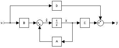
状態空間 (じょうたいくうかん、英 : State Space )あるいは状態空間表現 (じょうたいくうかんひょうげん、英 : State Space Representation )は、制御工学 において、物理的システムを入力と出力と状態変数を使った一階連立微分方程式 で表した数学的モデルである。入力、出力、状態は複数存在することが多いため、これらの変数はベクトルとして表され、行列形式で微分代数方程式を表す(力学系 が線形で時不変の場合)。状態空間表現は時間領域 の手法であり、これを使うと複数の入力と出力を持つシステムをコンパクトにモデル化でき、解析が容易になる。周波数領域 では、 p {\displaystyle p} q {\displaystyle q} q × p {\displaystyle q\times p} ラプラス変換 を書かなければならない。周波数領域の手法とは異なり、状態空間表現では、線形性と初期値がゼロという制限は存在しない。「状態空間」は、その次元軸が個々の状態変数に対応することから名づけられている。システムの状態はこの空間内のベクトルとして表現される。
典型的な状態空間モデル 状態変数は、任意の時点でシステム全体の状態を表せるシステム変数群の最小の部分集合である。状態変数群は線形独立でなければならない。すなわち、ある状態変数を別の状態変数群の線形結合で表すことはできない。システムを表現するのに必要な状態変数の最小個数 n {\displaystyle n} コンデンサ やコイル )の個数と同じであることが多い(常にそうとは限らない)。
p {\displaystyle p} q {\displaystyle q} n {\displaystyle n}
x ˙ ( t ) = A ( t ) x ( t ) + B ( t ) u ( t ) {\displaystyle {\dot {\mathbf {x} }}(t)=A(t)\mathbf {x} (t)+B(t)\mathbf {u} (t)} y ( t ) = C ( t ) x ( t ) + D ( t ) u ( t ) {\displaystyle \mathbf {y} (t)=C(t)\mathbf {x} (t)+D(t)\mathbf {u} (t)}
ここで、
x ( ⋅ ) {\displaystyle x(\cdot )} y ( ⋅ ) {\displaystyle y(\cdot )} u ( ⋅ ) {\displaystyle u(\cdot )} A ( ⋅ ) {\displaystyle A(\cdot )} B ( ⋅ ) {\displaystyle B(\cdot )} C ( ⋅ ) {\displaystyle C(\cdot )} D ( ⋅ ) {\displaystyle D(\cdot )} D ( ⋅ ) {\displaystyle D(\cdot )} t {\displaystyle t} t ∈ R {\displaystyle t\in \mathbb {R} } t ∈ Z {\displaystyle t\in \mathbb {Z} } k {\displaystyle k}
系の種類 状態空間モデル 連続時不変 x ˙ ( t ) = A x ( t ) + B u ( t ) {\displaystyle {\dot {\mathbf {x} }}(t)=A\mathbf {x} (t)+B\mathbf {u} (t)} y ( t ) = C x ( t ) + D u ( t ) {\displaystyle \mathbf {y} (t)=C\mathbf {x} (t)+D\mathbf {u} (t)} 連続時変 x ˙ ( t ) = A ( t ) x ( t ) + B ( t ) u ( t ) {\displaystyle {\dot {\mathbf {x} }}(t)=\mathbf {A} (t)\mathbf {x} (t)+\mathbf {B} (t)\mathbf {u} (t)} y ( t ) = C ( t ) x ( t ) + D ( t ) u ( t ) {\displaystyle \mathbf {y} (t)=\mathbf {C} (t)\mathbf {x} (t)+\mathbf {D} (t)\mathbf {u} (t)} 離散時不変 x ( k + 1 ) = A x ( k ) + B u ( k ) {\displaystyle \mathbf {x} (k+1)=A\mathbf {x} (k)+B\mathbf {u} (k)} y ( k ) = C x ( k ) + D u ( k ) {\displaystyle \mathbf {y} (k)=C\mathbf {x} (k)+D\mathbf {u} (k)} 離散時変 x ( k + 1 ) = A ( k ) x ( k ) + B ( k ) u ( k ) {\displaystyle \mathbf {x} (k+1)=\mathbf {A} (k)\mathbf {x} (k)+\mathbf {B} (k)\mathbf {u} (k)} y ( k ) = C ( k ) x ( k ) + D ( k ) u ( k ) {\displaystyle \mathbf {y} (k)=\mathbf {C} (k)\mathbf {x} (k)+\mathbf {D} (k)\mathbf {u} (k)} 連続時不変の s X ( s ) = A X ( s ) + B U ( s ) {\displaystyle s\mathbf {X} (s)=A\mathbf {X} (s)+B\mathbf {U} (s)} Y ( s ) = C X ( s ) + D U ( s ) {\displaystyle \mathbf {Y} (s)=C\mathbf {X} (s)+D\mathbf {U} (s)} 離散時不変の z X ( z ) = A X ( z ) + B U ( z ) {\displaystyle z\mathbf {X} (z)=A\mathbf {X} (z)+B\mathbf {U} (z)} Y ( z ) = C X ( z ) + D U ( z ) {\displaystyle \mathbf {Y} (z)=C\mathbf {X} (z)+D\mathbf {U} (z)}
システムのさまざまな特性(可制御性、可観測性、安定性)は、行列 A 、B 、C とD に決められる。
連続時不変状態空間モデルの伝達関数 は、次のように導出できる。
まず、次の式
x ˙ ( t ) = A x ( t ) + B u ( t ) {\displaystyle {\dot {\mathbf {x} }}(t)=A\mathbf {x} (t)+B\mathbf {u} (t)}
のラプラス変換 を求める。
s X ( s ) = A X ( s ) + B U ( s ) {\displaystyle s\mathbf {X} (s)=A\mathbf {X} (s)+B\mathbf {U} (s)}
次に X ( s ) {\displaystyle \mathbf {X} (s)}
( s I − A ) X ( s ) = B U ( s ) {\displaystyle (s\mathbf {I} -A)\mathbf {X} (s)=B\mathbf {U} (s)} X ( s ) = ( s I − A ) − 1 B U ( s ) {\displaystyle \mathbf {X} (s)=(s\mathbf {I} -A)^{-1}B\mathbf {U} (s)}
これを使って、出力方程式の X ( s ) {\displaystyle \mathbf {X} (s)}
Y ( s ) = C X ( s ) + D U ( s ) {\displaystyle \mathbf {Y} (s)=C\mathbf {X} (s)+D\mathbf {U} (s)} Y ( s ) = C ( ( s I − A ) − 1 B U ( s ) ) + D U ( s ) {\displaystyle \mathbf {Y} (s)=C((s\mathbf {I} -A)^{-1}B\mathbf {U} (s))+D\mathbf {U} (s)}
となる。伝達関数 G ( s ) {\displaystyle \mathbf {G} (s)}
G ( s ) = Y ( s ) / U ( s ) {\displaystyle \mathbf {G} (s)=\mathbf {Y} (s)/\mathbf {U} (s)}
従って、上で求めた Y ( s ) {\displaystyle \mathbf {Y} (s)} U ( s ) {\displaystyle \mathbf {U} (s)}
G ( s ) = C ( s I − A ) − 1 B + D = C a d j ( s I − A ) d e t ( s I − A ) B + D {\displaystyle \mathbf {G} (s)=C(s\mathbf {I} -A)^{-1}B+D=C{\frac {\mathrm {adj} (s\mathbf {I} -A)}{\mathrm {det} (s\mathbf {I} -A)}}B+D}
式の中には、 d e t ( s I − A ) {\displaystyle \mathrm {det} (s\mathbf {I} -A)} s I − A {\displaystyle sI-A} 行列式 であり、 a d j ( s I − A ) {\displaystyle \mathrm {adj} (s\mathbf {I} -A)} s I − A {\displaystyle sI-A} 余因子行列 である。
G ( s ) {\displaystyle \mathbf {G} (s)} q {\displaystyle q} × {\displaystyle \times } p {\displaystyle p} q p {\displaystyle qp} q {\displaystyle q}
なお、 d e t ( s I − A ) {\displaystyle \mathrm {det} (s\mathbf {I} -A)} 特性多項式 と呼ばれる。その多項式の根(固有値 )から、システムの伝達関数の極が得られる。それらの極を使って、そのシステムの安定性を解析できる。 G ( s ) {\displaystyle {\textbf {G}}(s)}
( s I − A ) − 1 {\displaystyle (s\mathbf {I} -A)^{-1}} アルゴリズム がある。
( s I − A ) − 1 = a d j ( s I − A ) d e t ( s I − A ) = ∑ k = 0 n − 1 Q k s k s n + a n − 1 s n − 1 + ⋯ + a 1 s + a 0 {\displaystyle {\begin{aligned}(s\mathbf {I} -A)^{-1}&={\frac {\mathrm {adj} (s\mathbf {I} -A)}{\mathrm {det} (s\mathbf {I} -A)}}\\&={\frac {\sum _{k=0}^{n-1}\mathbf {Q} _{k}s^{k}}{s^{n}+a_{n-1}s^{n-1}+\cdots +a_{1}s+a_{0}}}\end{aligned}}}
その中には、
または
0 = Q 0 A + a 0 I = A Q 0 + a 0 I {\displaystyle \mathbf {0} =\mathbf {Q} _{0}\mathbf {A} +a_{0}\mathbf {I} =\mathbf {AQ} _{0}+a_{0}\mathbf {I} }
最後の等式は、前の演算の精度を検査することができる。
プロパーな伝達関数(「厳密にプロパー」ではない)の実現も容易に得られる。その場合伝達関数を、厳密にプロパーな部分と定数部分という2つの部分に分割するというトリックを用いる。
G ( s ) = G S P ( s ) + G ( ∞ ) {\displaystyle {\textbf {G}}(s)={\textbf {G}}_{SP}(s)+{\textbf {G}}(\infty )}
厳密にプロパーな伝達関数は上述した方法で正準状態空間実現に変換できる。定数の状態空間実現が y ( t ) = G ( ∞ ) u ( t ) {\displaystyle {\textbf {y}}(t)={\textbf {G}}(\infty ){\textbf {u}}(t)} A , B , C の状態空間実現は厳密にプロパーな部分から得られ、行列 D は定数部分から得られる。
もう少し判りやすくするため、例を挙げて説明する。
G ( s ) = s 2 + 3 s + 3 s 2 + 2 s + 1 = s + 2 s 2 + 2 s + 1 + 1 {\displaystyle {\textbf {G}}(s)={\frac {s^{2}+3s+3}{s^{2}+2s+1}}={\frac {s+2}{s^{2}+2s+1}}+1}
この伝達関数から、次の可制御実現が得られる。
x ˙ ( t ) = [ − 2 − 1 1 0 ] x ( t ) + [ 1 0 ] u ( t ) {\displaystyle {\dot {\textbf {x}}}(t)={\begin{bmatrix}-2&-1\\1&0\\\end{bmatrix}}{\textbf {x}}(t)+{\begin{bmatrix}1\\0\end{bmatrix}}{\textbf {u}}(t)}
y ( t ) = [ 1 2 ] x ( t ) + [ 1 ] u ( t ) {\displaystyle {\textbf {y}}(t)={\begin{bmatrix}1&2\end{bmatrix}}{\textbf {x}}(t)+{\begin{bmatrix}1\end{bmatrix}}{\textbf {u}}(t)}
出力が入力に直接依存している点に注意されたい。これは伝達関数の G ( ∞ ) {\displaystyle {\textbf {G}}(\infty )}
従って、状態の可制御性(controllability)条件は、許容範囲内の入力で、ある有限の時間をかければ状態をある初期値から特定の値へと変化させることが可能であることを暗に示している。連続時不変状態空間モデルが制御可能 (controllable)であるとは、次が成り立つ場合である。
rank [ B A B A 2 B . . . A n − 1 B ] = n {\displaystyle \operatorname {rank} {\begin{bmatrix}B&AB&A^{2}B&...&A^{n-1}B\end{bmatrix}}=n}
可観測性(observability)とは、システムの外部出力を観測することでシステムの内部状態を推測可能かどうかの尺度である。システムの可観測性と可制御性は数学的な双対である。
連続時不変状態空間モデルが観測可能 (observable)であるとは、次が成り立つ場合である。
rank [ C C A . . . C A n − 1 ] = n {\displaystyle \operatorname {rank} {\begin{bmatrix}C\\CA\\...\\CA^{n-1}\end{bmatrix}}=n}
なお、Rank とは行列内の線形独立な列の数である。
厳密にプロパー(strictly proper)な伝達関数は、次のようにして容易に状態空間に変換可能である。
伝達関数を展開して分子と分母の全ての係数を明らかにする。これは、次のような形式になる。
G ( s ) = n 1 s 3 + n 2 s 2 + n 3 s + n 4 s 4 + d 1 s 3 + d 2 s 2 + d 3 s + d 4 {\displaystyle {\textbf {G}}(s)={\frac {n_{1}s^{3}+n_{2}s^{2}+n_{3}s+n_{4}}{s^{4}+d_{1}s^{3}+d_{2}s^{2}+d_{3}s+d_{4}}}}
これらの係数を以下のように直接に状態空間モデルに挿入できる。
x ˙ ( t ) = [ − d 1 − d 2 − d 3 − d 4 1 0 0 0 0 1 0 0 0 0 1 0 ] x ( t ) + [ 1 0 0 0 ] u ( t ) {\displaystyle {\dot {\textbf {x}}}(t)={\begin{bmatrix}-d_{1}&-d_{2}&-d_{3}&-d_{4}\\1&0&0&0\\0&1&0&0\\0&0&1&0\end{bmatrix}}{\textbf {x}}(t)+{\begin{bmatrix}1\\0\\0\\0\\\end{bmatrix}}{\textbf {u}}(t)}
y ( t ) = [ n 1 n 2 n 3 n 4 ] x ( t ) {\displaystyle {\textbf {y}}(t)={\begin{bmatrix}n_{1}&n_{2}&n_{3}&n_{4}\end{bmatrix}}{\textbf {x}}(t)}
この状態空間実現を可制御正準形式 (controllable canonical form)と呼ぶ。「可制御」とされるのは、得られるモデルが可制御であることが保証されているためである。
伝達関数の係数を使って、次のような正準形式も構築可能である。
x ˙ ( t ) = [ − d 1 1 0 0 − d 2 0 1 0 − d 3 0 0 1 − d 4 0 0 0 ] x ( t ) + [ n 1 n 2 n 3 n 4 ] u ( t ) {\displaystyle {\dot {\textbf {x}}}(t)={\begin{bmatrix}-d_{1}&1&0&0\\-d_{2}&0&1&0\\-d_{3}&0&0&1\\-d_{4}&0&0&0\end{bmatrix}}{\textbf {x}}(t)+{\begin{bmatrix}n_{1}\\n_{2}\\n_{3}\\n_{4}\end{bmatrix}}{\textbf {u}}(t)}
y ( t ) = [ 1 0 0 0 ] x ( t ) {\displaystyle {\textbf {y}}(t)={\begin{bmatrix}1&0&0&0\end{bmatrix}}{\textbf {x}}(t)}
この状態空間実現を可観測正準形式 (observable canonical form)と呼ぶ。「可観測」とされるのは、得られるモデルが可観測であることが保証されているためである。
安定性については、外部的な安定に関するBIBO安定性があり、内部的な安定に関するリアプノフ安定性と漸近安定性など平衡状態 の安定性もある。非線形システム の平衡状態は唯一ではないが、線形システム の状態行列A(t) が可逆的であるとき平衡状態が 0 {\displaystyle \mathbf {0} }
BIBO安定性はシステムの零状態応答を着目し、平衡状態の安定性はシステムの零入力応答を着目する。なお、リアプノフ安定性は、力学系 の安定性理論の基礎である。安定性の判定には、状態行列A との密接な関係がある。
BIBO安定性は、入力は有界するとき出力は必ず有界であること。これは、不安定な極がゼロによって打ち消される場合と考えられる。
システムをプロパーな伝達関数 G ( s ) = d e t ( s I − A ) {\displaystyle \mathrm {G} (s)=\mathrm {det} (s\mathbf {I} -A)}
状態空間の原点はリアプノフ安定の平衡状態である上に、次を満たす δ ( t 0 ) > 0 {\displaystyle \delta (t_{0})>0} t 0 {\displaystyle t_{0}}
‖ x ( t 0 ) ‖ < δ ( t 0 ) ⇒ lim t → ∞ ‖ x ( t ) ‖ = 0 {\displaystyle \|x(t_{0})\|<\delta (t_{0})\Rightarrow \lim _{t\to \infty }\|x(t)\|=0}
δ ( t 0 ) {\displaystyle \delta (t_{0})} t 0 {\displaystyle t_{0}} 一様漸近安定 状態という。
LTIシステム が漸近安定する必要十分条件は、システムの固有値(A の固有値)がすべて負の実部を持つ。
漸近安定のシステムは必ずBIBO安定する。 システムが可制御性または可観測性持たないとき、伝達関数の極が状態行列A のスペクトル(固有値の集)の真部分集合であるため、BIBO安定は必ず漸近安定ではない。でも、 LTIシステムには可制御性と可観測性が同時にあるとき、以下の命題が等価である。 システムがBIBO安定する。 システムが漸近安定する。 伝達関数の極が負の実部を持つ。 システムの固有値(A の固有値)が負の実部を持つ。
フィードバックのある典型的な状態空間モデル 典型的なフィードバックは、出力に行列 K をかけたものをシステムの入力とする。 system: u ( t ) = K y ( t ) {\displaystyle \mathbf {u} (t)=K\mathbf {y} (t)} K 内の値には制限はないので、負の値することで容易にネガティブ・フィードバック(負帰還)となる。負の符号は単に表記上の問題であって、式にそれが現われなくとも最終的な結果には何の影響もない。
x ˙ ( t ) = A x ( t ) + B u ( t ) {\displaystyle {\dot {\mathbf {x} }}(t)=A\mathbf {x} (t)+B\mathbf {u} (t)} y ( t ) = C x ( t ) + D u ( t ) {\displaystyle \mathbf {y} (t)=C\mathbf {x} (t)+D\mathbf {u} (t)}
この式の入力をフィードバックに置き換えると次の式になる。
x ˙ ( t ) = A x ( t ) + B K y ( t ) {\displaystyle {\dot {\mathbf {x} }}(t)=A\mathbf {x} (t)+BK\mathbf {y} (t)} y ( t ) = C x ( t ) + D K y ( t ) {\displaystyle \mathbf {y} (t)=C\mathbf {x} (t)+DK\mathbf {y} (t)}
出力方程式を y ( t ) {\displaystyle \mathbf {y} (t)}
x ˙ ( t ) = ( A + B K ( I − D K ) − 1 C ) x ( t ) {\displaystyle {\dot {\mathbf {x} }}(t)=\left(A+BK\left(I-DK\right)^{-1}C\right)\mathbf {x} (t)} y ( t ) = ( I − D K ) − 1 C x ( t ) {\displaystyle \mathbf {y} (t)=\left(I-DK\right)^{-1}C\mathbf {x} (t)}
この場合の利点は、 ( A + B K ( I − D K ) − 1 C ) {\displaystyle \left(A+BK\left(I-DK\right)^{-1}C\right)} K を適切に設定することで A の固有値 を制御できる点である。これは、開ループ系が制御可能 であるか、または A の不安定な固有値を K を適切に設定することで安定にできるということを前提としている。
比較的一般的な単純化として、D を除去し、C を単位元にすると、次のような式が得られる。
x ˙ ( t ) = ( A + B K ) x ( t ) {\displaystyle {\dot {\mathbf {x} }}(t)=\left(A+BK\right)\mathbf {x} (t)} y ( t ) = x ( t ) {\displaystyle \mathbf {y} (t)=\mathbf {x} (t)}
こうすると、固有値分解は A + B K {\displaystyle A+BK}
基準入力のある出力フィードバック フィードバックに加えて、入力 r ( t ) {\displaystyle r(t)} u ( t ) = − K y ( t ) + r ( t ) {\displaystyle \mathbf {u} (t)=-K\mathbf {y} (t)+\mathbf {r} (t)}
x ˙ ( t ) = A x ( t ) + B u ( t ) {\displaystyle {\dot {\mathbf {x} }}(t)=A\mathbf {x} (t)+B\mathbf {u} (t)} y ( t ) = C x ( t ) + D u ( t ) {\displaystyle \mathbf {y} (t)=C\mathbf {x} (t)+D\mathbf {u} (t)}
この式に当てはめると、次のようになる。
x ˙ ( t ) = A x ( t ) − B K y ( t ) + B r ( t ) {\displaystyle {\dot {\mathbf {x} }}(t)=A\mathbf {x} (t)-BK\mathbf {y} (t)+B\mathbf {r} (t)} y ( t ) = C x ( t ) − D K y ( t ) + D r ( t ) {\displaystyle \mathbf {y} (t)=C\mathbf {x} (t)-DK\mathbf {y} (t)+D\mathbf {r} (t)}
出力方程式を y ( t ) {\displaystyle \mathbf {y} (t)}
x ˙ ( t ) = ( A − B K ( I + D K ) − 1 C ) x ( t ) + B ( I − K ( I + D K ) − 1 D ) r ( t ) {\displaystyle {\dot {\mathbf {x} }}(t)=\left(A-BK\left(I+DK\right)^{-1}C\right)\mathbf {x} (t)+B\left(I-K\left(I+DK\right)^{-1}D\right)\mathbf {r} (t)} y ( t ) = ( I + D K ) − 1 C x ( t ) + ( I + D K ) − 1 D r ( t ) {\displaystyle \mathbf {y} (t)=\left(I+DK\right)^{-1}C\mathbf {x} (t)+\left(I+DK\right)^{-1}D\mathbf {r} (t)}
比較的一般的な単純化として、D を除去すると、次のような式が得られる。
x ˙ ( t ) = ( A − B K C ) x ( t ) + B r ( t ) {\displaystyle {\dot {\mathbf {x} }}(t)=\left(A-BKC\right)\mathbf {x} (t)+B\mathbf {r} (t)} y ( t ) = C x ( t ) {\displaystyle \mathbf {y} (t)=C\mathbf {x} (t)}
古典的な線形システムとして、一次元の移動する物体を考える。壁にバネで繋がれた物体が水平な平面上を移動する場合、ニュートン力学 では次の式で表される。
m y ¨ ( t ) = u ( t ) − k 1 y ˙ ( t ) − k 2 y ( t ) {\displaystyle m{\ddot {y}}(t)=u(t)-k_{1}{\dot {y}}(t)-k_{2}y(t)}
ここで
y ( t ) {\displaystyle y(t)} y ˙ ( t ) {\displaystyle {\dot {y}}(t)} y ¨ ( t ) {\displaystyle {\ddot {y}}(t)} u ( t ) {\displaystyle u(t)} k 1 {\displaystyle k_{1}} k 2 {\displaystyle k_{2}} m {\displaystyle m} この場合の状態方程式は次のようになる。
[ x 1 ˙ ( t ) x 2 ˙ ( t ) ] = [ 0 1 − k 2 m − k 1 m ] [ x 1 ( t ) x 2 ( t ) ] + [ 0 1 m ] u ( t ) {\displaystyle \left[{\begin{matrix}\mathbf {\dot {x_{1}}} (t)\\\mathbf {\dot {x_{2}}} (t)\end{matrix}}\right]=\left[{\begin{matrix}0&1\\-{\frac {k_{2}}{m}}&-{\frac {k_{1}}{m}}\end{matrix}}\right]\left[{\begin{matrix}\mathbf {x_{1}} (t)\\\mathbf {x_{2}} (t)\end{matrix}}\right]+\left[{\begin{matrix}0\\{\frac {1}{m}}\end{matrix}}\right]\mathbf {u} (t)} y ( t ) = [ 1 0 ] [ x 1 ( t ) x 2 ( t ) ] {\displaystyle \mathbf {y} (t)=\left[{\begin{matrix}1&0\end{matrix}}\right]\left[{\begin{matrix}\mathbf {x_{1}} (t)\\\mathbf {x_{2}} (t)\end{matrix}}\right]}
ここで、
x 1 ( t ) {\displaystyle x_{1}(t)} x 2 ( t ) := x 1 ˙ ( t ) {\displaystyle x_{2}(t):={\dot {x_{1}}}(t)} x 2 ˙ ( t ) = x 1 ¨ ( t ) {\displaystyle {\dot {x_{2}}}(t)={\ddot {x_{1}}}(t)} 出力 y ( t ) {\displaystyle \mathbf {y} (t)} 可制御性を評価すると、次のようになる。
[ B A B ] = [ [ 0 1 m ] [ 0 1 − k 2 m − k 1 m ] [ 0 1 m ] ] = [ 0 1 m 1 m k 1 m 2 ] {\displaystyle \left[{\begin{matrix}B&AB\end{matrix}}\right]=\left[{\begin{matrix}\left[{\begin{matrix}0\\{\frac {1}{m}}\end{matrix}}\right]&\left[{\begin{matrix}0&1\\-{\frac {k_{2}}{m}}&-{\frac {k_{1}}{m}}\end{matrix}}\right]\left[{\begin{matrix}0\\{\frac {1}{m}}\end{matrix}}\right]\end{matrix}}\right]=\left[{\begin{matrix}0&{\frac {1}{m}}\\{\frac {1}{m}}&{\frac {k_{1}}{m^{2}}}\end{matrix}}\right]}
したがって、 k 1 {\displaystyle k_{1}} m {\displaystyle m}
可観測性を評価すると、次のようになる。
[ C C A ] = [ [ 1 0 ] [ 1 0 ] [ 0 1 − k 2 m − k 1 m ] ] = [ 1 0 0 1 ] {\displaystyle \left[{\begin{matrix}C\\CA\end{matrix}}\right]=\left[{\begin{matrix}\left[{\begin{matrix}1&0\end{matrix}}\right]\\\left[{\begin{matrix}1&0\end{matrix}}\right]\left[{\begin{matrix}0&1\\-{\frac {k_{2}}{m}}&-{\frac {k_{1}}{m}}\end{matrix}}\right]\end{matrix}}\right]=\left[{\begin{matrix}1&0\\0&1\end{matrix}}\right]}
したがって、フルランクである。以上から、このシステムは制御可能で、かつ観測可能である。
より普遍的な状態空間モデルの形式は次のように表される。
x ˙ ( t ) = f ( t , x ( t ) , u ( t ) ) {\displaystyle \mathbf {\dot {x}} (t)=\mathbf {f} (t,x(t),u(t))} y ( t ) = h ( t , x ( t ) , u ( t ) ) {\displaystyle \mathbf {y} (t)=\mathbf {h} (t,x(t),u(t))}
1つ目が状態方程式、2つ目が出力方程式である。 f ( ⋅ , ⋅ , ⋅ ) {\displaystyle f(\cdot ,\cdot ,\cdot )} u ( t ) {\displaystyle u(t)}
古典的な非線形システムとして、力を加えない単純な振り子 を考える。
m l θ ¨ ( t ) = − m g sin θ ( t ) − k l θ ˙ ( t ) {\displaystyle ml{\ddot {\theta }}(t)=-mg\sin \theta (t)-kl{\dot {\theta }}(t)}
ここで、
θ ( t ) {\displaystyle \theta (t)} m {\displaystyle m} g {\displaystyle g} k {\displaystyle k} l {\displaystyle l} m {\displaystyle m} すると、状態方程式は次のようになる。
x 1 ˙ ( t ) = x 2 ( t ) {\displaystyle {\dot {x_{1}}}(t)=x_{2}(t)} x 2 ˙ ( t ) = − g l sin x 1 ( t ) − k m x 2 ( t ) {\displaystyle {\dot {x_{2}}}(t)=-{\frac {g}{l}}\sin {x_{1}}(t)-{\frac {k}{m}}{x_{2}}(t)}
ここで、
x 1 ( t ) := θ ( t ) {\displaystyle x_{1}(t):=\theta (t)} x 2 ( t ) := x 1 ˙ ( t ) {\displaystyle x_{2}(t):={\dot {x_{1}}}(t)} x 2 ˙ = x 1 ¨ {\displaystyle {\dot {x_{2}}}={\ddot {x_{1}}}} 状態方程式は、次のようにも書き表せる。
x ˙ ( t ) = ( x 1 ˙ ( t ) x 2 ˙ ( t ) ) = f ( t , x ( t ) ) = ( x 2 ( t ) − g l sin x 1 ( t ) − k m x 2 ( t ) ) {\displaystyle {\dot {x}}(t)=\left({\begin{matrix}{\dot {x_{1}}}(t)\\{\dot {x_{2}}}(t)\end{matrix}}\right)=\mathbf {f} (t,x(t))=\left({\begin{matrix}x_{2}(t)\\-{\frac {g}{l}}\sin {x_{1}}(t)-{\frac {k}{m}}{x_{2}}(t)\end{matrix}}\right)}
システムの平衡/安定点は x ˙ = 0 {\displaystyle {\dot {x}}=0}
( x 1 x 2 ) = ( n π 0 ) {\displaystyle \left({\begin{matrix}x_{1}\\x_{2}\end{matrix}}\right)=\left({\begin{matrix}n\pi \\0\end{matrix}}\right)}
ここで n は整数である。
Chen, Chi-Tsong 1999. Linear System Theory and Design , 3rd. ed., Oxford University Press (ISBN 0-19-511777-8) Khalil, Hassan K. Nonlinear Systems , 3rd. ed., Prentice Hall (ISBN 0-13-067389-7) Nise, Norman S. 2004. Control Systems Engineering , 4th ed., John Wiley & Sons, Inc. (ISBN 0-471-44577-0) Hinrichsen, Diederich and Pritchard, Anthony J. 2005. Mathematical Systems Theory I, Modelling, State Space Analysis, Stability and Robustness . Springer. (ISBN 978-3-540-44125-0) Sontag, Eduardo D. 1999. Mathematical Control Theory: Deterministic Finite Dimensional Systems. Second Edition . Springer. (ISBN 0-387-984895) (フリーなオンライン版) Durbin, J. and S. Koopman (2001). Time series analysis by state space methods . Oxford University Press, Oxford. 状態空間の考え方を計量経済学 に応用したもの 分野 系特性 デジタル制御 先進技術 制御器 制御応用


![{\displaystyle \operatorname {dim} [A(\cdot )]=n\times n}](https://wikimedia.org/api/rest_v1/media/math/render/svg/cdb067922e2d625e2d0aaab3b6e54239cdd4f759)
![{\displaystyle \operatorname {dim} [B(\cdot )]=n\times p}](https://wikimedia.org/api/rest_v1/media/math/render/svg/e273a2878042f414ada7b454096d2d66125257a6)
![{\displaystyle \operatorname {dim} [C(\cdot )]=q\times n}](https://wikimedia.org/api/rest_v1/media/math/render/svg/6aa4ac576864f9f09ea580fb19bd480fd12a68be)
![{\displaystyle \operatorname {dim} [D(\cdot )]=q\times p}](https://wikimedia.org/api/rest_v1/media/math/render/svg/759072ec7232e15a1823aec56b668df529d57dee)


![{\displaystyle \left[{\begin{matrix}\mathbf {\dot {x_{1}}} (t)\\\mathbf {\dot {x_{2}}} (t)\end{matrix}}\right]=\left[{\begin{matrix}0&1\\-{\frac {k_{2}}{m}}&-{\frac {k_{1}}{m}}\end{matrix}}\right]\left[{\begin{matrix}\mathbf {x_{1}} (t)\\\mathbf {x_{2}} (t)\end{matrix}}\right]+\left[{\begin{matrix}0\\{\frac {1}{m}}\end{matrix}}\right]\mathbf {u} (t)}](https://wikimedia.org/api/rest_v1/media/math/render/svg/0bde243f9d17f91b1d03020e9559e8120fae677f)
![{\displaystyle \mathbf {y} (t)=\left[{\begin{matrix}1&0\end{matrix}}\right]\left[{\begin{matrix}\mathbf {x_{1}} (t)\\\mathbf {x_{2}} (t)\end{matrix}}\right]}](https://wikimedia.org/api/rest_v1/media/math/render/svg/089622c024d88e55fb7da811b54574235a1af4a1)


![{\displaystyle \left[{\begin{matrix}B&AB\end{matrix}}\right]=\left[{\begin{matrix}\left[{\begin{matrix}0\\{\frac {1}{m}}\end{matrix}}\right]&\left[{\begin{matrix}0&1\\-{\frac {k_{2}}{m}}&-{\frac {k_{1}}{m}}\end{matrix}}\right]\left[{\begin{matrix}0\\{\frac {1}{m}}\end{matrix}}\right]\end{matrix}}\right]=\left[{\begin{matrix}0&{\frac {1}{m}}\\{\frac {1}{m}}&{\frac {k_{1}}{m^{2}}}\end{matrix}}\right]}](https://wikimedia.org/api/rest_v1/media/math/render/svg/8085052653d9c3f6548abce458f14b47264c544f)
![{\displaystyle \left[{\begin{matrix}C\\CA\end{matrix}}\right]=\left[{\begin{matrix}\left[{\begin{matrix}1&0\end{matrix}}\right]\\\left[{\begin{matrix}1&0\end{matrix}}\right]\left[{\begin{matrix}0&1\\-{\frac {k_{2}}{m}}&-{\frac {k_{1}}{m}}\end{matrix}}\right]\end{matrix}}\right]=\left[{\begin{matrix}1&0\\0&1\end{matrix}}\right]}](https://wikimedia.org/api/rest_v1/media/math/render/svg/379549fbd631c3d00cff027b1208378f396a65e0)


